Stan と R でベイズ統計モデリング 第四章
math python r stanTable of Contents
#+File Created:
#+Last Updated:
Stan と R でベイズ統計モデリング (第四章)の学習記録
この本は素晴らしい. めちゃんこ賢い人が書いた本って感じがする.
疑問に思いそうなところをちゃんと先回りしてわかりやすく解説してくれているし,
書き方に統一感があって, 読み進めていくうちに自然に身につくような構成となっている.
この本では RStan を使った解説が行われているが,
これからは cmdstanr/cmdstanpy らしい( Cmdstanr入門とreduce_sum()解説 ) のでこれらを用いて書き直してみる.
基礎となる単回帰の説明がある第四章を見てみる.
自分用メモ.
1 Stan の基本的文法
1.1 ブロック構成
Stan の最も簡単なプログラム例.
データ Y は正規分布する.
求めたいパラメータは平均値 mu. の場合.
 1: data {
 2:   int N;
 3:   real Y[N];
 4: }
 5:
 6: parameters {
 7:   real mu;
 8: }
 9:
10: model {
11:   for(i in 1:N) {
12:     Y[N] ~ normal(mu,1)
13:   }
14:   mu ~ normal(0,100);
15: }
1.2 コーディング規約
- インデント
- データ変数は大文字から, パラメータは小文字から始める.
- ブロックの間は1行あける.
- 変数名は snake_case にする.
- ~ 及び = の前後はスペースあける.
2 Stan の lp__ と target
事後確率は以下のように計算できる.
$$
p(\theta|Y) \propto p(Y|\theta) p(\theta)
$$
対数事後確率は
$$
\log p(\theta|Y) \propto \log p(Y|\theta) + \log p(\theta)
$$
Stan の結果データの中に出てくる lp__ (log posterior) は, 各 MCMC step でパラメータ \(\theta\) に何か具体的な値 \(\theta^{\star}\) を入れたときの \(\log p(\theta^{\star}|Y)\) の値.
$$
lp\_\_ = \log p(\theta^{\star}|Y) \propto \log p(Y|\theta^{\star}) + \log p(\theta^{\star})
$$
データが \(N\) 個あれば以下のようになる. もちろん \(Y_i\) には何らかの具体的な数値が入っている.
$$
lp\_\_ = \log p(\theta^{\star}|Y) \propto \sum_{i=1}^{N} \log p(Y_i|\theta^{\star}) + \log p(\theta^{\star})
$$
Stan の model ブロックでの \(Y \sim dist(\theta)\) という書き方は,
内部的には以下のように計算されている.
1: lp__ = log(p(theta));   # 事前分布(の log)
2: for(i in 1:N) {
3:   lp__ += log(p(Y[i]|theta));  # データは独立なので確率を掛け算(log なので足し算になる)
4: }
target は lp__ の別名である.
Stan では, target に \(\log p(Y|\theta)\) を足し込んでいく上のような書き方が出来るようになっている.
特に複雑な尤度計算を行う際にはこっちの書き方をする場合がある.
普通の書き方
1: model {
2:   for(i in 1:N) {
3:     Y[i] ~ normal(mu,1);
4:   }
5:   mu ~ normal(0,100);
6: }
を target に足し込む形式で書くと以下のようになる.
normal_ldf(Y[i]|mu, sigma) は \(\log normal(Y[i]|\mu, sigma)\) を表す便利な関数.
(ldf は log probability density function. log 確率密度関数)
1: model {
2:   for(i in 1:N) {
3:     target += normal_lpdf(Y[i]|mu,1);
4:   }
5:   target += normal_lpdf(mu|0,100);
6: }
3 単回帰
これが全ての基礎. よくわかんなくなったらここに戻ってくること.
単回帰の例で Stan 及び cmdstanr/cmdstanpy の典型的な使い方を見てみる.
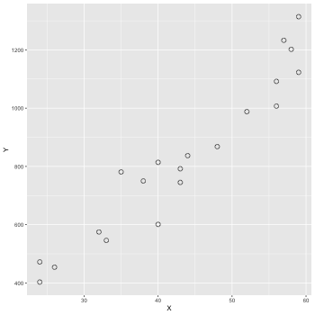
3.1 データの図示
データファイル: data-salary.txt (X 列, Y 列がある. X 列の値から Y の値をよそくしたい!!)
ggplot2 で図を描いてみる.
1: library(ggplot2)
2: d <- read.csv(file='data-salary.txt')
3: p <- ggplot(data=d) + geom_point(mapping=aes(x=X,y=Y),shape=1, size=3)
4: fname <- '04_01_fig.png'
5: ggsave(file=fname, plot=p, dpi=50)   # dpi で図の大きさ(解像度)を指定
3.2 単回帰(lm)
lm 関数を使って単回帰を行う.
1: d <- read.csv(file='data-salary.txt')
2: res <- lm(Y ~ X, data=d)
3: summary(res)
Call:
lm(formula = Y ~ X, data = d)

Residuals:
     Min       1Q   Median       3Q      Max
-155.471  -51.523   -6.663   52.822  141.349

Coefficients:
            Estimate Std. Error t value Pr(>|t|)
(Intercept) -119.697     68.148  -1.756    0.096 .
X             21.904      1.518  14.428 2.47e-11 ***
---
Signif. codes:  0 ‘***’ 0.001 ‘**’ 0.01 ‘*’ 0.05 ‘.’ 0.1 ‘ ’ 1

Residual standard error: 79.1 on 18 degrees of freedom
Multiple R-squared:  0.9204,	Adjusted R-squared:  0.916
F-statistic: 208.2 on 1 and 18 DF,  p-value: 2.466e-11
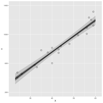
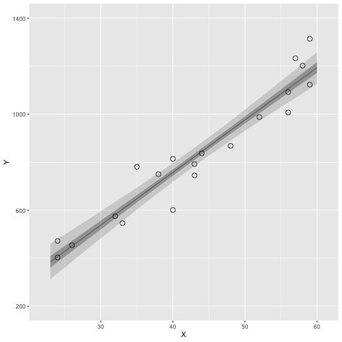
信頼区間
coord_cartesian(xlim=Xの範囲, ylim=Yの範囲)
scale_y_continuous() で Y の補助目盛りの設定など
 1: d <- read.csv(file='data-salary.txt')
 2: res <- lm(Y ~ X, data=d)
 3:
 4: X_new <- data.frame(X=23:60)
 5: conf_95 <- predict(res, X_new, interval='confidence', level=0.95)
 6: conf_50 <- predict(res, X_new, interval='confidence', level=0.50)
 7: conf_95 <- data.frame(X_new,conf_95)  # 列名 = (X,fit,lwr,upr)
 8: conf_50 <- data.frame(X_new,conf_50)
 9:
10: library(ggplot2)
11: p <- ggplot()
12: p <- p + geom_ribbon(data=conf_95, mapping=aes(x=X,ymin=lwr,ymax=upr), alpha=1/6)
13: p <- p + geom_ribbon(data=conf_50, mapping=aes(x=X,ymin=lwr,ymax=upr), alpha=3/6)
14: p <- p + geom_line(data=conf_50,aes(x=X,y=fit),size=1) # 線
15: p <- p + geom_point(data=d, aes(x=X, y=Y), shape=1, size=3) # まる
16: p <- p + labs(x='X', y='Y') + coord_cartesian(xlim=c(22, 61), ylim=c(200, 1400))
17: p <- p + scale_y_continuous(breaks=seq(from=200, to=1400, by=400))
18: fname <- 'fig4-3-left.png'
19: ggsave(file=fname, plot=p, dpi=50)
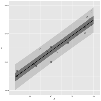
予測区間を描く.
confidence –> prediction にする.
 1: d <- read.csv(file='data-salary.txt')
 2: res <- lm(Y ~ X, data=d)
 3:
 4: X_new <- data.frame(X=23:60)
 5: pred_95 <- predict(res, X_new, interval='prediction', level=0.95)
 6: pred_50 <- predict(res, X_new, interval='prediction', level=0.50)
 7: pred_95 <- data.frame(X_new,pred_95)  # 列名 = (X,fit,lwr,upr)
 8: pred_50 <- data.frame(X_new,pred_50)
 9:
10: library(ggplot2)
11: p <- ggplot()
12: p <- p + geom_ribbon(data=pred_95, mapping=aes(x=X,ymin=lwr,ymax=upr), alpha=1/6)
13: p <- p + geom_ribbon(data=pred_50, mapping=aes(x=X,ymin=lwr,ymax=upr), alpha=3/6)
14: p <- p + geom_line(data=pred_50,aes(x=X,y=fit),size=1) # 線
15: p <- p + geom_point(data=d, aes(x=X, y=Y), shape=1, size=3) # まる
16: p <- p + labs(x='X', y='Y') + coord_cartesian(xlim=c(22, 61), ylim=c(200, 1400))
17: p <- p + scale_y_continuous(breaks=seq(from=200, to=1400, by=400))
18: fname <- 'fig4-3-right.png'
19: ggsave(file=fname, plot=p, dpi=50)
3.3 Stan で実装 (1) cmdstanr
 1: data {
 2:   int N;
 3:   real X[N];
 4:   real Y[N];
 5: }
 6:
 7: parameters {
 8:   real a;
 9:   real b;
10:   real<lower=0> sigma;
11: }
12:
13: model {
14:   for(i in 1:N) {
15:     Y[i] ~ normal(a + b*X[i], sigma);
16:   }
17: }
これをキックする R コードを書く.
本にある RStan ではなく comdstanr で書いてみる.
1: library(cmdstanr)
2: d <- read.csv(file='data-salary.txt')
3: data <- list(N=nrow(d), X=d$X, Y=d$Y)
4: model  <- cmdstan_model('model4-5.stan')
5: fit <- model$sample(data=data, chains=4, parallel_chains=4, seed=1234)
6: fit$save_output_files(dir="./", basename='model4-5', timestamp=FALSE, random=FALSE)
Running MCMC with 4 parallel chains...

Chain 1 Iteration:    1 / 2000 [  0%]  (Warmup)
...
Chain 1 Iteration: 1001 / 2000 [ 50%]  (Sampling)
Chain 1 Iteration: 1100 / 2000 [ 55%]  (Sampling)
Chain 1 Iteration: 1200 / 2000 [ 60%]  (Sampling)
Chain 1 Iteration: 1300 / 2000 [ 65%]  (Sampling)
Chain 1 Iteration: 1400 / 2000 [ 70%]  (Sampling)
Chain 1 Iteration: 1500 / 2000 [ 75%]  (Sampling)
Chain 1 Iteration: 1600 / 2000 [ 80%]  (Sampling)
Chain 1 Iteration: 1700 / 2000 [ 85%]  (Sampling)
Chain 1 Iteration: 1800 / 2000 [ 90%]  (Sampling)
Chain 1 Iteration: 1900 / 2000 [ 95%]  (Sampling)
Chain 1 Iteration: 2000 / 2000 [100%]  (Sampling)
.....
Chain 4 Iteration: 1700 / 2000 [ 85%]  (Sampling)
Chain 4 Iteration: 1800 / 2000 [ 90%]  (Sampling)
Chain 4 Iteration: 1900 / 2000 [ 95%]  (Sampling)
Chain 4 Iteration: 2000 / 2000 [100%]  (Sampling)
Chain 1 finished in 0.1 seconds.
Chain 2 finished in 0.1 seconds.
Chain 3 finished in 0.1 seconds.
Chain 4 finished in 0.1 seconds.

All 4 chains finished successfully.
Mean chain execution time: 0.1 seconds.
Total execution time: 0.3 seconds.
csv ファイルからの読み込み
結果を見てみる.
Read CmdStan CSV files into R — read_cmdstan_csv • cmdstanr
1: library(cmdstanr)
2: files <- c('model4-5-1.csv',
3:            'model4-5-2.csv',
4:            'model4-5-3.csv',
5:            'model4-5-4.csv')
6: fit <- as_cmdstan_fit(files)
7: fit$summary()
# A tibble: 4 × 10
  variable   mean median    sd   mad     q5    q95  rhat ess_bulk ess_tail
  <chr>     <dbl>  <dbl> <dbl> <dbl>  <dbl>  <dbl> <dbl>    <dbl>    <dbl>
1 lp__      -93.6  -93.3  1.26  1.04  -96.1 -92.2   1.01    1304.    1691.
2 a        -117.  -119.  71.3  68.7  -236.    2.08  1.00    1377.    1556.
3 b          21.9   21.9  1.60  1.54   19.2  24.5   1.00    1349.    1501.
4 sigma      84.5   82.4 15.2  14.3    63.8 112.    1.01    1615.    1361.
lm では a = -119.7, b = 21.9 と推定されていたのでほぼ同じ結果が出たと言って良いだろう.
RStan の形式で見るには以下のようにする.
1: library(rstan)
2: files <-c('model4-5-1.csv',
3:           'model4-5-2.csv',
4:           'model4-5-3.csv',
5:           'model4-5-4.csv')
6: rstanfit <- rstan::read_stan_csv(files)  # rstan の fit object が作成できた. これを使う.
7: options(width=180)
8: summary(rstanfit)$summary
            mean    se_mean        sd       2.5%        25%        50%       75%     97.5%    n_eff     Rhat
a     -117.45496 1.93495619 71.307379 -257.65965 -164.64975 -119.17350 -71.97750  23.16816 1358.084 1.000974
b       21.85965 0.04379069  1.597700   18.67989   20.82737   21.88625  22.90630  24.97104 1331.149 1.001300
sigma   84.50608 0.40945078 15.213551   61.08729   73.71800   82.41410  93.17735 120.02752 1380.568 1.005035
lp__   -93.60737 0.03683109  1.256416  -96.86346  -94.18972  -93.27450 -92.69150 -92.13598 1163.691 1.007309
3.4 Stan 結果解析
MCMC データの extract は fit$draws
1: library(cmdstanr)
2: files <- c('model4-5-1.csv',
3:            'model4-5-2.csv',
4:            'model4-5-3.csv',
5:            'model4-5-4.csv')
6: fit <- as_cmdstan_fit(files)
7: ms <- fit$draws(format='matrix')  # chain を一つにまとめる
8: dim(ms)
9: head(ms)
[1] 4000    4
# A draws_matrix: 6 iterations, 1 chains, and 4 variables
    variable
draw lp__      a  b sigma
   1  -93  -94.6 21    72
   2  -93  -79.0 21    87
   3  -94  -34.5 21    95
   4  -93  -50.5 20    96
   5  -94    6.4 19    90
   6  -92 -133.7 22    81
パラメータの分布を図示
 1: library(cmdstanr)
 2: library(ggplot2)
 3: files <- c('model4-5-1.csv',
 4:            'model4-5-2.csv',
 5:            'model4-5-3.csv',
 6:            'model4-5-4.csv')
 7: fit <- as_cmdstan_fit(files)
 8: p <- bayesplot::mcmc_dens(fit$draws(c('a','b','sigma')))
 9: fname <- 'model4-5_param_dens.png'
10: ggsave(file=fname, plot=p, dpi=70)
ヒストグラムで描くと
 1: library(cmdstanr)
 2: library(ggplot2)
 3: files <- c('model4-5-1.csv',
 4:            'model4-5-2.csv',
 5:            'model4-5-3.csv',
 6:            'model4-5-4.csv')
 7: fit <- as_cmdstan_fit(files)
 8: p <- bayesplot::mcmc_hist(fit$draws(c('a','b','sigma')))
 9: fname <- 'model4-5_param_hist.png'
10: ggsave(file=fname, plot=p, dpi=70)
trace plot
 1: library(cmdstanr)
 2: library(ggplot2)
 3: files <- c('model4-5-1.csv',
 4:            'model4-5-2.csv',
 5:            'model4-5-3.csv',
 6:            'model4-5-4.csv')
 7: fit <- as_cmdstan_fit(files)
 8: p <- bayesplot::mcmc_trace(fit$draws(c('a','b','sigma')))
 9: fname <- 'model4-5_param_trace.png'
10: ggsave(file=fname, plot=p, dpi=70)
mcmc_dens_overlay
chain ごとに描く.
 1: library(cmdstanr)
 2: library(ggplot2)
 3: files <- c('model4-5-1.csv',
 4:            'model4-5-2.csv',
 5:            'model4-5-3.csv',
 6:            'model4-5-4.csv')
 7: fit <- as_cmdstan_fit(files)
 8: p <- bayesplot::mcmc_dens_overlay(fit$draws(c('a','b','sigma')))
 9: fname <- 'model4-5_param_dens_overlay.png'
10: ggsave(file=fname, plot=p, dpi=70)

mcmc_pairs
パラメータ間の関係をみる.
 1: library(cmdstanr)
 2: library(ggplot2)
 3: files <- c('model4-5-1.csv',
 4:            'model4-5-2.csv',
 5:            'model4-5-3.csv',
 6:            'model4-5-4.csv')
 7: fit <- as_cmdstan_fit(files)
 8: p <- bayesplot::mcmc_pairs(fit$draws(c('a','b')))
 9: fname <- 'model4-5_param_pairs.png'
10: ggsave(file=fname, plot=p, dpi=70)
 1: library(cmdstanr)
 2: files <- c('model4-5-1.csv',
 3:            'model4-5-2.csv',
 4:            'model4-5-3.csv',
 5:            'model4-5-4.csv')
 6: fit <- as_cmdstan_fit(files)
 7: ms <- fit$draws(format='df')
 8: head(ms)
 9: head(ms$a)
10: length(ms$a)
11: quantile(ms$b, probs=c(0.025,0.975))
# A draws_df: 6 iterations, 1 chains, and 4 variables
  lp__      a  b sigma
1  -93  -94.6 21    72
2  -93  -79.0 21    87
3  -94  -34.5 21    95
4  -93  -50.5 20    96
5  -94    6.4 19    90
6  -92 -133.7 22    81
# ... hidden reserved variables {'.chain', '.iteration', '.draw'}
[1]  -94.58260  -79.03710  -34.45430  -50.53660    6.44861 -133.72600
[1] 4000
    2.5%    97.5%
18.67989 24.97104
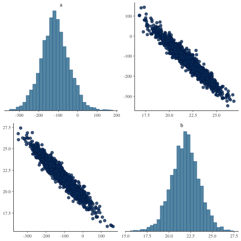
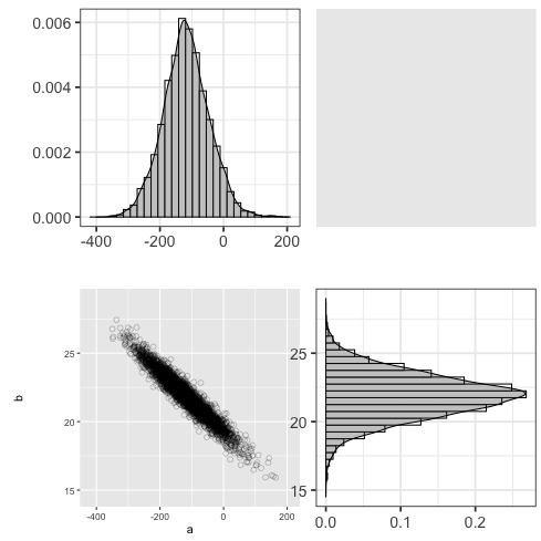
mcmc_pairs に似た図を ggplot を用いて描いてみる
 1: library(ggplot2)
 2: library(cmdstanr)
 3: files <- c('model4-5-1.csv',
 4:            'model4-5-2.csv',
 5:            'model4-5-3.csv',
 6:            'model4-5-4.csv')
 7: fit <- as_cmdstan_fit(files)
 8: df_mcmc <- fit$draws(format='df')
 9: # 散布図
10: p_xy <- ggplot(df_mcmc,aes(x=a,y=b)) +
11:     geom_point(alpha=1/4,size=2,shape=1) +
12:     scale_x_continuous(breaks=seq(-400,200,200), limits=c(-420,210)) +
13:     scale_y_continuous(breaks=seq(15,25,5),limits=c(14.5,29))
14:
15: # a の分布図
16: p_x <- ggplot(df_mcmc,aes(x=a)) + theme_bw(base_size=18) + theme(legend.position='none') +
17:     geom_histogram(aes(y=..density..),color='black',fill='white') +
18:     geom_density(alpha=0.3,fill='gray20') +
19:     scale_x_continuous(breaks=seq(-400,200,200),limits=c(-420,210))+
20:     labs(x='',y='')
21: # b の分布図
22: p_y <- ggplot(df_mcmc, aes(x=b)) + theme_bw(base_size=18) + theme(legend.position='none') +
23:     coord_flip() +
24:     geom_histogram(aes(y=..density..), colour='black', fill='white') +
25:     geom_density(alpha=0.3, fill='gray20') +
26:     scale_x_continuous(breaks=seq(15, 25, 5), limits=c(14.5, 29)) +
27:     labs(x='', y='')
28:
29: p_emp <- ggplot(data.frame(0,0)) + theme(rect=element_rect(fill='white'), panel.border=element_blank())
30:
31: g_xy  <- ggplotGrob(p_xy)
32: g_x   <- ggplotGrob(p_x)
33: g_y   <- ggplotGrob(p_y)
34: g_emp <- ggplotGrob(p_emp)
35:
36: g1 <- cbind(g_x,  g_emp, size='first')
37: g2 <- cbind(g_xy, g_y,   size='first')
38: g  <- rbind(g1,   g2,    size='first')
39: fname <- 'fig4-7.png'
40: ggsave(file=fname, plot=g, dpi=70)
3.5 ベイズ信頼区間
ベイズ信頼区間(R の中での計算の例)
 1: library(ggplot2)
 2: library(cmdstanr)
 3: files <- c('model4-5-1.csv',
 4:            'model4-5-2.csv',
 5:            'model4-5-3.csv',
 6:            'model4-5-4.csv')
 7: fit <- as_cmdstan_fit(files)
 8: ms <- fit$draws(format='df')
 9:
10: X_new <- 23:60
11: N_X <- length(X_new)
12: N_mcmc <- length(ms$lp__)
13:
14: set.seed(1234)
15: y_base_mcmc <- as.data.frame(matrix(nrow=N_mcmc,ncol=N_X))
16: y_mcmc      <- as.data.frame(matrix(nrow=N_mcmc,ncol=N_X))
17:
18: # i 列目のデータを作る
19: for (i in 1:N_X) {
20:     y_base_mcmc[,i] <- ms$a + ms$b * X_new[i]
21:     y_mcmc[,i]      <- rnorm(n=N_mcmc,mean=y_base_mcmc[,i],sd=ms$sigma)
22: }
23: conf <- data.frame(X=X_new,t(apply(y_base_mcmc,2,quantile,probs=c(0.025,0.25,0.50,0.75,0.975))))
24: colnames(conf) <- c('X','p025','p250','p500','p750','p975')
25:
26: d <- read.csv(file='data-salary.txt')
27: p <- ggplot()
28: p <- p + geom_ribbon(data=conf,aes(x=X,ymin=p025,ymax=p975),alpha=1/6)
29: p <- p + geom_ribbon(data=conf,aes(x=X,ymin=p250,ymax=p750),alpha=2/6)
30: p <- p + geom_line(  data=conf,aes(x=X,y=p500),size=0.2) # 線
31: p <- p + geom_point( data=d,   aes(x=X,y=Y), shape=1, size=3) # まる
32: p <- p + labs(x='X', y='Y') + coord_cartesian(xlim=c(22, 61), ylim=c(200, 1400))
33: p <- p + scale_y_continuous(breaks=seq(from=200, to=1400, by=400))
34:
35: fname <- 'fig4-8-left.png'
36: ggsave(file=fname, plot=p, dpi=70)
3.6 ベイズ予測区間
ベイズ予測区間(R の中での計算の例)
 1: library(ggplot2)
 2: library(cmdstanr)
 3: files <- c('model4-5-1.csv',
 4:            'model4-5-2.csv',
 5:            'model4-5-3.csv',
 6:            'model4-5-4.csv')
 7: fit <- as_cmdstan_fit(files)
 8: ms <- fit$draws(format='df')
 9:
10: X_new <- 23:60
11: N_X <- length(X_new)
12: N_mcmc <- length(ms$lp__)
13:
14: set.seed(1234)
15: y_base_mcmc <- as.data.frame(matrix(nrow=N_mcmc,ncol=N_X))
16: y_mcmc      <- as.data.frame(matrix(nrow=N_mcmc,ncol=N_X))
17:
18: # i 列目のデータを作る
19: for (i in 1:N_X) {
20:     y_base_mcmc[,i] <- ms$a + ms$b * X_new[i]
21:     y_mcmc[,i]      <- rnorm(n=N_mcmc,mean=y_base_mcmc[,i],sd=ms$sigma)
22: }
23:
24: # y_base_mcmc --> y_mcmc に変更しただけ
25: conf <- data.frame(X=X_new,t(apply(y_mcmc,2,quantile,probs=c(0.025,0.25,0.50,0.75,0.975))))
26: colnames(conf) <- c('X','p025','p250','p500','p750','p975')
27:
28: d <- read.csv(file='data-salary.txt')
29: p <- ggplot()
30: p <- p + geom_ribbon(data=conf,aes(x=X,ymin=p025,ymax=p975),alpha=1/6)
31: p <- p + geom_ribbon(data=conf,aes(x=X,ymin=p250,ymax=p750),alpha=2/6)
32: p <- p + geom_line(  data=conf,aes(x=X,y=p500),size=0.2) # 線
33: p <- p + geom_point( data=d,   aes(x=X,y=Y), shape=1, size=3) # まる
34: p <- p + labs(x='X', y='Y') + coord_cartesian(xlim=c(22, 61), ylim=c(200, 1400))
35: p <- p + scale_y_continuous(breaks=seq(from=200, to=1400, by=400))
36:
37: fname <- 'fig4-8-right.png'
38: ggsave(file=fname, plot=p, dpi=70)

3.7 transformed parametes 及び generated quantities ブロック
処理は出来るだけ Stan 側でやらせたい.
R では出てきたデータの解析と図示に使う.
ベイズ信頼区間, 予測区間など, サンプルから派生する乱数計算部分を Stan に任せる.
(model4-4.stan)
data {
  int N;
  real X[N];
  real Y[N];
  // 追加部分
  int N_new;
  real X_new[N_new];
}

parameters {
  real a;
  real b;
  real<lower=0> sigma;
}

// transformed parameters では,
// data, parameter を組み合わせて,
// 新しいサンプリングパラメータを作成出来る.
transformed parameters {
  real y_base[N];
  for (i in 1:N) {
    y_base[i] = a + b*X[i];
  }
}

model {
  for (i in 1:N) {
    Y[i] ~ normal(y_base[i],sigma);
  }
}

// generated quantities では,
// data, parameter, transformed parameter を使って,
// 新しいサンプリングパラメータを作成出来る.
// 分布に従う乱数作成の際には, ~ ではなく
// y = 分布名_rng(parameter) という形で = で代入する点に注意する.
generated quantities {
  real y_base_new[N_new];
  real y_new[N_new];
  for (i in 1:N_new) {
    y_base_new[i] = a + b*X_new[i];
    y_new[i]      = normal_rng(y_base_new[i],sigma);
  }
}
cmdstanr を用いてキックする R code を作成する.
library(cmdstanr)
d     <- read.csv(file="data-salary.txt")
X_new <- 23:60
data  <- list(N=nrow(d),X=d$X,Y=d$Y,N_new=length(X_new),X_new=X_new)
model <- cmdstan_model('model4-4.stan')
fit   <- model$sample(data=data, chains=4, parallel_chains=4, seed=1234)
fit$save_output_files(dir="./", basename='model4-4', timestamp=FALSE, random=FALSE)
Running MCMC with 4 parallel chains...

Chain 1 Iteration:    1 / 2000 [  0%]  (Warmup)
Chain 1 Iteration:  100 / 2000 [  5%]  (Warmup)
Chain 1 Iteration:  200 / 2000 [ 10%]  (Warmup)
....
Chain 4 Iteration: 1400 / 2000 [ 70%]  (Sampling)
Chain 4 Iteration: 1500 / 2000 [ 75%]  (Sampling)
Chain 4 Iteration: 1600 / 2000 [ 80%]  (Sampling)
Chain 4 Iteration: 1700 / 2000 [ 85%]  (Sampling)
Chain 4 Iteration: 1800 / 2000 [ 90%]  (Sampling)
Chain 4 Iteration: 1900 / 2000 [ 95%]  (Sampling)
Chain 4 Iteration: 2000 / 2000 [100%]  (Sampling)
Chain 1 finished in 0.1 seconds.
Chain 2 finished in 0.1 seconds.
Chain 3 finished in 0.1 seconds.
Chain 4 finished in 0.1 seconds.

All 4 chains finished successfully.
Mean chain execution time: 0.1 seconds.
Total execution time: 0.3 seconds.
ちょっとテスト. df の中身を確認.
1: library(cmdstanr)
2: files <- c('model4-4-1.csv',
3:            'model4-4-2.csv',
4:            'model4-4-3.csv',
5:            'model4-4-4.csv')
6: fit <- as_cmdstan_fit(files)
7: df <- fit$summary(variables=c('y_base_new'),'mean','sd', 'quantile', 'rhat','ess_bulk','ess_tail')
8: head(df)
# A tibble: 6 × 11
  variable     mean    sd  `0%` `25%` `50%` `75%` `100%`  rhat ess_bulk ess_tail
  <chr>       <dbl> <dbl> <dbl> <dbl> <dbl> <dbl>  <dbl> <dbl>    <dbl>    <dbl>
1 y_base_new…  386.  40.9  217.  360.  386.  412.   575.  1.00    1366.    1353.
2 y_base_new…  408.  39.3  246.  383.  407.  432.   588.  1.00    1382.    1303.
3 y_base_new…  429.  37.8  274.  405.  429.  453.   602.  1.00    1401.    1419.
4 y_base_new…  451.  36.3  303.  428.  451.  474.   616.  1.00    1421.    1414.
5 y_base_new…  473.  34.9  331.  451.  473.  495.   630.  1.00    1444.    1395.
6 y_base_new…  495.  33.4  359.  474.  495.  516.   644.  1.00    1473.    1438.
 1: library(cmdstanr)
 2: q95 <- function(x) quantile(x, probs=c(0.025, 0.25, 0.5, 0.75, 0.975))
 3: files <- c('model4-4-1.csv',
 4:            'model4-4-2.csv',
 5:            'model4-4-3.csv',
 6:            'model4-4-4.csv')
 7: fit <- as_cmdstan_fit(files)
 8: df <- fit$summary(variables=c('y_base_new'),'mean','sd', q95)
 9: X_new <- 23:60
10: df$X_new <- X_new
11: print(df)
12: print(class(df$"50%"))  # 書き出すときはこれでもOKだが.
13: print(df$`50%`)  # ggplot の aes で使うときは `50%` (back quote?) を使う
14: print(X_new)
# A tibble: 38 × 9
   variable        mean    sd `2.5%` `25%` `50%` `75%` `97.5%` X_new
   <chr>          <dbl> <dbl>  <dbl> <dbl> <dbl> <dbl>   <dbl> <int>
 1 y_base_new[1]   386.  40.9   305.  360.  386.  412.    466.    23
 2 y_base_new[2]   408.  39.3   329.  383.  407.  432.    485.    24
 3 y_base_new[3]   429.  37.8   354.  405.  429.  453.    504.    25
 4 y_base_new[4]   451.  36.3   379.  428.  451.  474.    522.    26
 5 y_base_new[5]   473.  34.9   403.  451.  473.  495.    541.    27
 6 y_base_new[6]   495.  33.4   428.  474.  495.  516.    561.    28
 7 y_base_new[7]   517.  32.0   453.  497.  516.  537.    580.    29
 8 y_base_new[8]   538.  30.7   477.  519.  538.  558.    599.    30
 9 y_base_new[9]   560.  29.3   502.  542.  560.  579.    619.    31
10 y_base_new[10]  582.  28.0   526.  564.  582.  600.    638.    32
# … with 28 more rows
[1] "numeric"
 [1]  385.5130  407.4335  429.0850  451.3160  472.9815  494.5715  516.3015
 [8]  537.9880  559.8315  581.7540  603.2995  625.3255  647.2970  669.3170
[15]  691.0870  713.0220  734.9595  756.7530  778.5770  800.3400  822.2360
[22]  844.0335  865.6885  887.4945  909.2655  931.0180  953.1985  975.1065
[29]  996.8525 1018.6000 1040.5050 1062.1500 1084.0350 1105.8150 1127.7300
[36] 1149.6500 1171.4100 1193.2600
 [1] 23 24 25 26 27 28 29 30 31 32 33 34 35 36 37 38 39 40 41 42 43 44 45 46 47
[26] 48 49 50 51 52 53 54 55 56 57 58 59 60
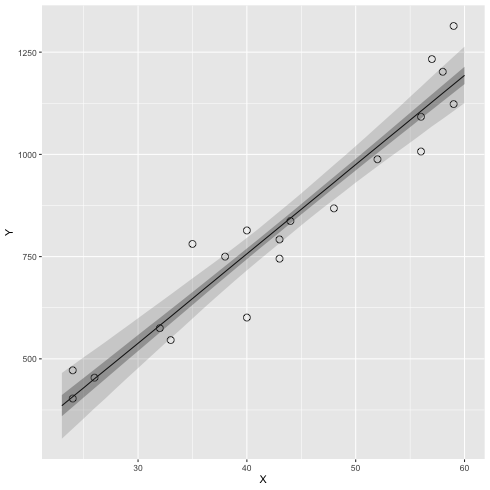
ベイズ信頼区間の図を描いてみる.
 1: library(cmdstanr)
 2: library(ggplot2)
 3:
 4: # 95% 信頼区間
 5: q95 <- function(x) quantile(x, probs=c(0.025, 0.25, 0.5, 0.75, 0.975))
 6: files <- c('model4-4-1.csv',
 7:            'model4-4-2.csv',
 8:            'model4-4-3.csv',
 9:            'model4-4-4.csv')
10: fit <- as_cmdstan_fit(files)
11: df <- fit$summary(variables=c('y_base_new'),'mean','sd', q95)
12: X_new <- 23:60
13: df$X_new <- X_new
14:
15: # 元データ
16: d     <- read.csv(file="data-salary.txt")
17:
18: # 図
19: p <- ggplot() + geom_point(data=d, mapping=aes(x=X,y=Y), shape=1, size=3)
20: p <- p + geom_line(data=df,mapping=aes(x=X_new,y=`50%`))
21: p <- p + geom_ribbon(data=df, mapping=aes(x=X_new, ymax=`97.5%`,ymin=`2.5%`),alpha=1/6)
22: p <- p + geom_ribbon(data=df, mapping=aes(x=X_new, ymax=`75%`  ,ymin=`25%` ),alpha=2/6)
23:
24: fname <- 'fig4-8-left_cmdstan.png'
25: ggsave(file=fname, plot=p, dpi=70)
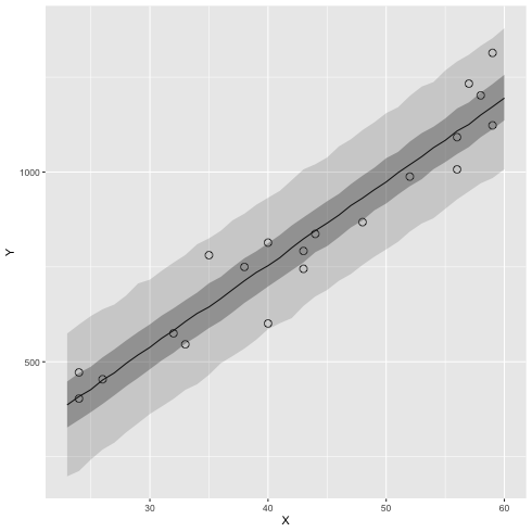
ベイズ予測区間
 1: library(cmdstanr)
 2: library(ggplot2)
 3:
 4: # 95% 信頼区間
 5: q95 <- function(x) quantile(x, probs=c(0.025, 0.25, 0.5, 0.75, 0.975))
 6: files <- c('model4-4-1.csv',
 7:            'model4-4-2.csv',
 8:            'model4-4-3.csv',
 9:            'model4-4-4.csv')
10: fit <- as_cmdstan_fit(files)
11: df <- fit$summary(variables=c('y_new'),'mean','sd', q95)
12: X_new <- 23:60
13: df$X_new <- X_new
14:
15: # 元データ
16: d     <- read.csv(file="data-salary.txt")
17:
18: # 図
19: p <- ggplot() + geom_point(data=d, mapping=aes(x=X,y=Y), shape=1, size=3)
20: p <- p + geom_line(data=df,mapping=aes(x=X_new,y=`50%`))
21: p <- p + geom_ribbon(data=df, mapping=aes(x=X_new, ymax=`97.5%`,ymin=`2.5%`),alpha=1/6)
22: p <- p + geom_ribbon(data=df, mapping=aes(x=X_new, ymax=`75%`  ,ymin=`25%` ),alpha=2/6)
23:
24: fname <- 'fig4-8-right_cmdstan.png'
25: ggsave(file=fname, plot=p, dpi=70)
3.8 Stan で実装(2) cmdstanpy
Stan code は generated quantities がある model4-4.stan を用いよう.
キックする Python script (cmdstanpy) を書く.
 1: import pandas as pd
 2: from cmdstanpy import CmdStanModel
 3:
 4: d = pd.read_csv("data-salary.txt",header=0)
 5: N = len(d)
 6: X = d.iloc[:,0]
 7: Y = d.iloc[:,1]
 8: X_new = range(23,61)
 9: N_new = len(X_new)
10: data = {'N': N, 'X': X,  'Y': Y, 'N_new': N_new, 'X_new': X_new}
11: model = CmdStanModel(stan_file='model4-4.stan',model_name='model4-4')
12: fit = model.sample(data=data, chains=4, parallel_chains=4, seed=1234)
13: # ファイル名を指定できない... timestamp とか要らないんだが.
14: fit.save_csvfiles(dir='./')
15: fpd = fit.summary()
16: print(fpd.head(50))
                  Mean   MCSE  StdDev      5%  ...     95%   N_Eff  N_Eff/s  R_hat
name                                           ...
lp__             -94.0  0.049     1.5   -96.0  ...   -92.0   910.0   3300.0    1.0
a               -120.0  2.300    79.0  -240.0  ...    10.0  1200.0   4400.0    1.0
b                 22.0  0.050     1.7    19.0  ...    25.0  1200.0   4400.0    1.0
sigma             85.0  0.460    16.0    64.0  ...   110.0  1300.0   4600.0    1.0
y_base[1]        408.0  1.100    39.0   345.0  ...   471.0  1337.0   4863.0    1.0
y_base[2]        408.0  1.100    39.0   345.0  ...   471.0  1337.0   4863.0    1.0
y_base[3]        451.0  0.980    36.0   394.0  ...   510.0  1376.0   5004.0    1.0
y_base[4]        582.0  0.700    28.0   537.0  ...   627.0  1598.0   5810.0    1.0
y_base[5]        604.0  0.660    27.0   561.0  ...   647.0  1667.0   6061.0    1.0
y_base[6]        648.0  0.570    25.0   608.0  ...   687.0  1859.0   6759.0    1.0
y_base[7]        713.0  0.440    22.0   677.0  ...   748.0  2443.0   8884.0    1.0
y_base[8]        757.0  0.360    20.0   723.0  ...   789.0  3216.0  11694.0    1.0
y_base[9]        757.0  0.360    20.0   723.0  ...   789.0  3216.0  11694.0    1.0
y_base[10]       822.0  0.300    19.0   791.0  ...   853.0  4285.0  15580.0    1.0
y_base[11]       822.0  0.300    19.0   791.0  ...   853.0  4285.0  15580.0    1.0
y_base[12]       844.0  0.290    19.0   812.0  ...   875.0  4461.0  16224.0    1.0
y_base[13]       931.0  0.320    21.0   897.0  ...   965.0  4192.0  15242.0    1.0
y_base[14]      1019.0  0.460    24.0   979.0  ...  1058.0  2781.0  10114.0    1.0
y_base[15]      1106.0  0.630    29.0  1058.0  ...  1154.0  2127.0   7734.0    1.0
y_base[16]      1106.0  0.630    29.0  1058.0  ...  1154.0  2127.0   7734.0    1.0
y_base[17]      1128.0  0.680    30.0  1078.0  ...  1178.0  2026.0   7367.0    1.0
y_base[18]      1150.0  0.720    32.0  1097.0  ...  1202.0  1941.0   7058.0    1.0
y_base[19]      1171.0  0.770    33.0  1117.0  ...  1226.0  1869.0   6796.0    1.0
y_base[20]      1171.0  0.770    33.0  1117.0  ...  1226.0  1869.0   6796.0    1.0
y_base_new[1]    386.0  1.100    41.0   320.0  ...   452.0  1322.0   4807.0    1.0
y_base_new[2]    408.0  1.100    39.0   345.0  ...   471.0  1337.0   4863.0    1.0
y_base_new[3]    429.0  1.000    38.0   370.0  ...   491.0  1355.0   4929.0    1.0
y_base_new[4]    451.0  0.980    36.0   394.0  ...   510.0  1376.0   5004.0    1.0
y_base_new[5]    473.0  0.930    35.0   418.0  ...   529.0  1400.0   5092.0    1.0
y_base_new[6]    495.0  0.890    33.0   442.0  ...   548.0  1427.0   5187.0    1.0
y_base_new[7]    517.0  0.840    32.0   466.0  ...   568.0  1458.0   5302.0    1.0
y_base_new[8]    538.0  0.790    31.0   489.0  ...   588.0  1496.0   5440.0    1.0
y_base_new[9]    560.0  0.750    29.0   514.0  ...   607.0  1542.0   5607.0    1.0
y_base_new[10]   582.0  0.700    28.0   537.0  ...   627.0  1598.0   5810.0    1.0
y_base_new[11]   604.0  0.660    27.0   561.0  ...   647.0  1667.0   6061.0    1.0
y_base_new[12]   626.0  0.610    26.0   585.0  ...   667.0  1752.0   6371.0    1.0
y_base_new[13]   648.0  0.570    25.0   608.0  ...   687.0  1859.0   6759.0    1.0
y_base_new[14]   669.0  0.530    23.0   631.0  ...   708.0  1996.0   7257.0    1.0
y_base_new[15]   691.0  0.480    23.0   654.0  ...   728.0  2191.0   7966.0    1.0
y_base_new[16]   713.0  0.440    22.0   677.0  ...   748.0  2443.0   8884.0    1.0
y_base_new[17]   735.0  0.400    21.0   700.0  ...   769.0  2771.0  10077.0    1.0
y_base_new[18]   757.0  0.360    20.0   723.0  ...   789.0  3216.0  11694.0    1.0
y_base_new[19]   779.0  0.330    20.0   746.0  ...   811.0  3615.0  13145.0    1.0
y_base_new[20]   800.0  0.310    20.0   768.0  ...   832.0  4045.0  14708.0    1.0
y_base_new[21]   822.0  0.300    19.0   791.0  ...   853.0  4285.0  15580.0    1.0
y_base_new[22]   844.0  0.290    19.0   812.0  ...   875.0  4461.0  16224.0    1.0
y_base_new[23]   866.0  0.290    20.0   834.0  ...   897.0  4526.0  16458.0    1.0
y_base_new[24]   888.0  0.300    20.0   855.0  ...   919.0  4470.0  16255.0    1.0
y_base_new[25]   909.0  0.310    20.0   876.0  ...   942.0  4314.0  15689.0    1.0
y_base_new[26]   931.0  0.320    21.0   897.0  ...   965.0  4192.0  15242.0    1.0

[50 rows x 9 columns]
csv ファイルからロードできる.
What is the proper way to save a cmdstanpy model after a fit has been complete? - General - The Stan Forums
API Reference — CmdStanPy 1.0.0rc1 documentation
API Reference — CmdStanPy 1.0.1 documentation
cmdstanpy – Python interface to CmdStan — CmdStanPy 1.0.1 documentation
 1: import cmdstanpy
 2: # 何か面倒
 3: files=['model4-4-20220331192118_1.csv',
 4:        'model4-4-20220331192118_2.csv',
 5:        'model4-4-20220331192118_3.csv',
 6:        'model4-4-20220331192118_4.csv']
 7: fit = cmdstanpy.from_csv(path=files, method='sample')
 8: df = fit.summary(percentiles=(2.5, 50, 97.5))
 9: print(type(df))   # pandas dataframe として保存されている様子.
10: print(df.head(5))
<class 'pandas.core.frame.DataFrame'>
            Mean   MCSE  StdDev   2.5%    50%  97.5%   N_Eff  N_Eff/s  R_hat
name
lp__       -94.0  0.049     1.5  -98.0  -93.0  -92.0   910.0   3100.0    1.0
a         -120.0  2.300    79.0 -290.0 -120.0   32.0  1200.0   4100.0    1.0
b           22.0  0.050     1.7   18.0   22.0   25.0  1200.0   4100.0    1.0
sigma       85.0  0.460    16.0   60.0   83.0  120.0  1300.0   4200.0    1.0
y_base[1]  408.0  1.100    39.0  323.0  407.0  482.0  1337.0   4503.0    1.0
cmdstanpy の計算結果 csv ファイルを R (cmdstanr) で読み込むことも可能
1: library(cmdstanr)
2: files <-c('model4-4-20220331192118_1.csv',
3:           'model4-4-20220331192118_2.csv',
4:           'model4-4-20220331192118_3.csv',
5:           'model4-4-20220331192118_4.csv')
6: fit <- as_cmdstan_fit(files)
7: fit$summary()
# A tibble: 100 × 10
   variable    mean median    sd   mad     q5    q95  rhat ess_bulk ess_tail
   <chr>      <dbl>  <dbl> <dbl> <dbl>  <dbl>  <dbl> <dbl>    <dbl>    <dbl>
 1 lp__       -93.7  -93.3  1.46  1.12  -96.5 -92.2   1.00    1133.    1216.
 2 a         -116.  -117.  78.6  74.3  -242.    9.99  1.00    1248.    1240.
 3 b           21.8   21.8  1.75  1.62   19.0  24.6   1.00    1253.    1232.
 4 sigma       85.3   82.9 16.4  14.2    63.7 114.    1.00    1523.    1343.
 5 y_base[1]  408.   407.  39.3  37.1   346.  471.    1.00    1382.    1303.
 6 y_base[2]  408.   407.  39.3  37.1   346.  471.    1.00    1382.    1303.
 7 y_base[3]  451.   451.  36.3  34.0   394.  510.    1.00    1421.    1414.
 8 y_base[4]  582.   582.  28.0  26.6   537.  627.    1.00    1662.    1715.
 9 y_base[5]  604.   603.  26.8  25.5   561.  647.    1.00    1736.    1745.
10 y_base[6]  648.   647.  24.5  23.1   608.  687.    1.00    1939.    1927.
# … with 90 more rows
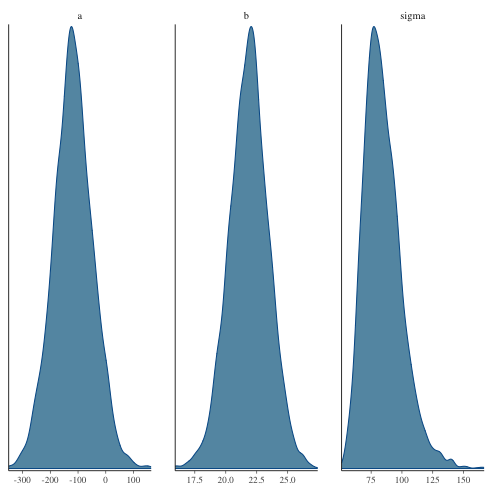
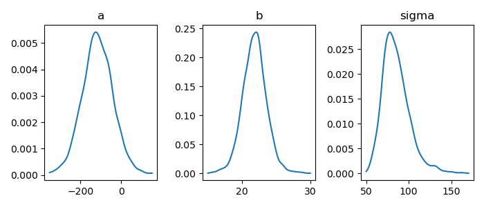
パラメータの分布(密度グラフ)
Matplotlib 密度プロット | Delft スタック
from scipy.stats import kde
density = kde.gaussian_kde(データ)
x = np.linspace(x最小, x最大, 分割数)
y = density(x) # 密度値の推定
ax.plot(x,y)
 1: import numpy as np
 2: import cmdstanpy
 3: import matplotlib.pyplot as plt
 4: from scipy.stats import kde
 5: files=['model4-4-20220331192118_1.csv',
 6:        'model4-4-20220331192118_2.csv',
 7:        'model4-4-20220331192118_3.csv',
 8:        'model4-4-20220331192118_4.csv']
 9: fit = cmdstanpy.from_csv(path=files, method='sample')
10:
11: la = fit.stan_variables()  # { a:[...], b:[...], y_base:[[....],[....],....] }
12: adraw = la['a']
13: bdraw = la['b']
14: sdraw = la['sigma']
15:
16: adens = kde.gaussian_kde(adraw)
17: x = np.linspace(-350,150,100)
18: y = adens(x)
19:
20: bdens = kde.gaussian_kde(bdraw)
21: bx = np.linspace(15,30,100)
22: by = bdens(bx)
23:
24: sdens = kde.gaussian_kde(sdraw)
25: sx = np.linspace(50,170,100)
26: sy = sdens(sx)
27:
28: fig = plt.figure(dpi=100, figsize=(7,3))
29: ax = fig.add_subplot(1,3,1)
30: ax.set_title('a')
31: ax.plot(x,y)
32: ax2 = fig.add_subplot(1,3,2)
33: ax2.set_title('b')
34: ax2.plot(bx,by)
35: ax3 = fig.add_subplot(1,3,3)
36: ax3.set_title('sigma')
37: ax3.plot(sx,sy)
38:
39: # plt.rcParams['font.size'] = 5
40: plt.tight_layout()
41:
42: fname = 'model4-5_param_dens_py.png'
43: fig.show()
44: fig.savefig(fname)
matplotlib でヒストグラムを描く – Python でデータサイエンス
ヒストグラムのパラメータ
plt.hist(x, bins=16) # 棒の数を 16 に
plt.hist(x, range(50,100)) # 50 - 100 まで
plt.hist(x, normed=True) # 正規化
plt.hist(x, rwidth=0.8) # 棒の幅
plt.hist(x, color="red") # 棒の色
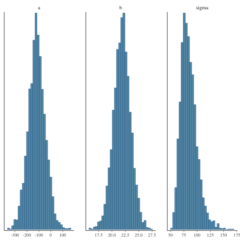
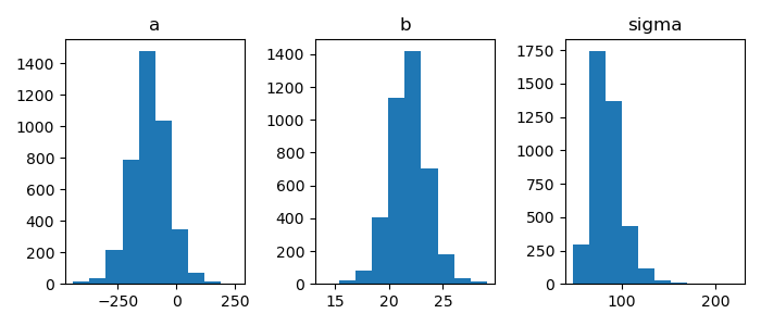
パラメータの分布(ヒストグラム)
 1: import numpy as np
 2: import cmdstanpy
 3: import matplotlib.pyplot as plt
 4: from scipy.stats import kde
 5: files=['model4-4-20220331192118_1.csv',
 6:        'model4-4-20220331192118_2.csv',
 7:        'model4-4-20220331192118_3.csv',
 8:        'model4-4-20220331192118_4.csv']
 9: fit = cmdstanpy.from_csv(path=files, method='sample')
10:
11: la = fit.stan_variables()  # { a:[...], b:[...], y_base:[[....],[....],....] }
12: adraw = la['a']
13: bdraw = la['b']
14: sdraw = la['sigma']
15:
16: fig = plt.figure(dpi=100, figsize=(7,3))
17: ax = fig.add_subplot(1,3,1)
18: ax.set_title('a')
19: ax.hist(adraw)
20: ax2 = fig.add_subplot(1,3,2)
21: ax2.set_title('b')
22: ax2.hist(bdraw)
23: ax3 = fig.add_subplot(1,3,3)
24: ax3.set_title('sigma')
25: ax3.hist(sdraw)
26:
27: # plt.rcParams['font.size'] = 5
28: plt.tight_layout()
29:
30: fname = 'model4-5_param_hist_py.png'
31: fig.show()
32: fig.savefig(fname)
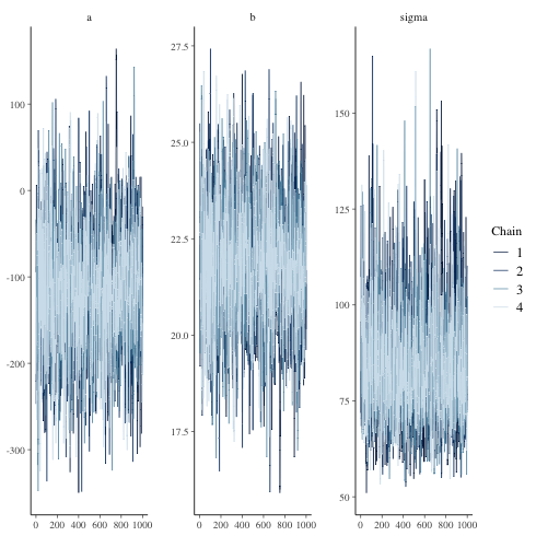
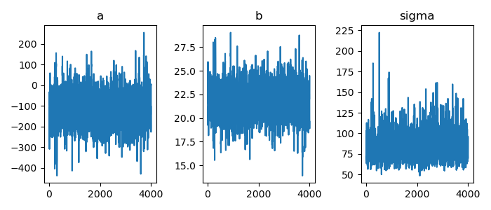
trace plot
 1: # テストプログラム
 2: import numpy as np
 3: import cmdstanpy
 4: import matplotlib.pyplot as plt
 5: from scipy.stats import kde
 6: files=['model4-4-20220331192118_1.csv',
 7:        'model4-4-20220331192118_2.csv',
 8:        'model4-4-20220331192118_3.csv',
 9:        'model4-4-20220331192118_4.csv']
10: fit = cmdstanpy.from_csv(path=files, method='sample')
11:
12: la = fit.stan_variables()  # { a:[...], b:[...], y_base:[[....],[....],....] }
13: adraw = la['a']
14: xmax = len(adraw)
15: print(xmax)
16: rng = range(0, xmax)
17: print(len(rng))
4000
4000
 1: import numpy as np
 2: import cmdstanpy
 3: import matplotlib.pyplot as plt
 4: from scipy.stats import kde
 5: files=['model4-4-20220331192118_1.csv',
 6:        'model4-4-20220331192118_2.csv',
 7:        'model4-4-20220331192118_3.csv',
 8:        'model4-4-20220331192118_4.csv']
 9: fit = cmdstanpy.from_csv(path=files, method='sample')
10:
11: la = fit.stan_variables()  # { a:[...], b:[...], y_base:[[....],[....],....] }
12: adraw = la['a']
13: bdraw = la['b']
14: sdraw = la['sigma']
15: x = range(0, len(adraw))
16:
17: fig = plt.figure(dpi=100, figsize=(7,3))
18: ax = fig.add_subplot(1,3,1)
19: ax.set_title('a')
20: ax.plot(x,adraw)
21: ax2 = fig.add_subplot(1,3,2)
22: ax2.set_title('b')
23: ax2.plot(x,bdraw)
24: ax3 = fig.add_subplot(1,3,3)
25: ax3.set_title('sigma')
26: ax3.plot(x,sdraw)
27:
28: # plt.rcParams['font.size'] = 5
29: plt.tight_layout()
30:
31: fname = 'model4-5_param_trace_py.png'
32: fig.show()
33: fig.savefig(fname)
ベイズ信頼区間
 1: # テストプログラム
 2: import numpy as np
 3: import cmdstanpy
 4: import matplotlib.pyplot as plt
 5: import pandas as pd
 6: d = pd.read_csv("data-salary.txt",header=0)
 7: print(len(d['X']))
 8: files=['model4-4-20220331192118_1.csv',
 9:        'model4-4-20220331192118_2.csv',
10:        'model4-4-20220331192118_3.csv',
11:        'model4-4-20220331192118_4.csv']
12: fit = cmdstanpy.from_csv(path=files, method='sample')
13:
14: la = fit.stan_variables()  # { a:[...], b:[...], y_base:[[....],[....],....] }
15: #print(type(la))   # dict
16: ybase = la['y_base']
17:
18: p = np.percentile(ybase[:,0], q=[2.5, 25, 50, 75, 97.5]) # [329.275975 382.54375  407.4335   432.47275  484.563225]
19: #print(p)
20: df = pd.DataFrame()
21: i = 42
22: df[23] = np.percentile(ybase[:,0], q=[2.5, 25, 50, 75, 97.5])
23: df[i] = np.percentile(ybase[:,i-23], q=[2.5, 25, 50, 75, 97.5])
24: # 転置
25: df2 = df.T
26: # 列名の設定
27: df3 = df2.set_axis(['p2.5','p25','p50','p75','p97.5'], axis='columns')
28: print(df3)
20
           p2.5         p25        p50         p75        p97.5
23   329.275975   382.54375   407.4335   432.47275   484.563225
42  1106.094250  1150.85000  1171.4100  1191.71000  1239.130500
pandas.DataFrameの行名・列名の変更 | note.nkmk.me
列名付け替え
df.set_axis(['col1', 'col2'], axis='columns')
 1: # テストプログラム2
 2: import numpy as np
 3: import cmdstanpy
 4: import matplotlib.pyplot as plt
 5: import pandas as pd
 6: d = pd.read_csv("data-salary.txt",header=0)
 7: X = d['X']
 8: files=['model4-4-20220331192118_1.csv',
 9:        'model4-4-20220331192118_2.csv',
10:        'model4-4-20220331192118_3.csv',
11:        'model4-4-20220331192118_4.csv']
12: fit = cmdstanpy.from_csv(path=files, method='sample')
13:
14: la = fit.stan_variables()  # { a:[...], b:[...], y_base:[[....],[....],....] }
15: ybase = la['y_base']
16: df = pd.DataFrame()
17: for i in range(0,len(X)):
18:     df[i] = np.percentile(ybase[:,i], q=[2.5, 25, 50, 75, 97.5])
19: df2 = df.T
20: df3 = df2.set_axis(['p2.5','p25','p50','p75','p97.5'], axis='columns')
21: print(df3)
           p2.5         p25        p50         p75        p97.5
0    329.275975   382.54375   407.4335   432.47275   484.563225
1    329.275975   382.54375   407.4335   432.47275   484.563225
2    379.150450   428.25850   451.3160   474.11425   522.375525
3    526.263225   564.34250   581.7540   599.98400   638.039400
4    550.385900   586.78125   603.2995   621.00875   657.497800
5    598.459200   631.78200   647.2970   663.10925   696.845625
6    670.206100   699.27075   713.0220   726.92225   755.416825
7    716.318075   743.69250   756.7530   769.93875   796.053550
8    716.318075   743.69250   756.7530   769.93875   796.053550
9    782.588625   809.31350   822.2360   834.73925   860.563200
10   782.588625   809.31350   822.2360   834.73925   860.563200
11   804.537575   831.35400   844.0335   856.57175   882.364875
12   889.549775   918.08100   931.0180   944.99675   974.112375
13   970.801500  1003.26750  1018.6000  1033.78250  1068.110500
14  1048.405500  1087.87750  1105.8150  1124.20000  1165.291000
15  1048.405500  1087.87750  1105.8150  1124.20000  1165.291000
16  1068.381250  1108.75000  1127.7300  1146.72250  1190.291000
17  1086.878250  1129.85000  1149.6500  1169.22750  1214.831250
18  1106.094250  1150.85000  1171.4100  1191.71000  1239.130500
19  1106.094250  1150.85000  1171.4100  1191.71000  1239.130500
pythonでグラフ上に白抜き○をプロットする : No Link No Life
Matplotlib で散布図のマーカーサイズを設定する方法 | Delft スタック
plt.scatter(x,y, marker='o', s=100, facecolor='None', edgecolor='black') # s は丸のサイズ
Matplotlibのみで線形回帰の信頼区間を描画する | 知識のサラダボウル
plt.fill_between(x, lower, upper, color='', alpha=0.4) こんな感じで描くことができそう
 1: import numpy as np
 2: import cmdstanpy
 3: import matplotlib.pyplot as plt
 4: import pandas as pd
 5: d = pd.read_csv("data-salary.txt",header=0)
 6: X = d['X']
 7: Y = d['Y']
 8: files=['model4-4-20220331192118_1.csv',
 9:        'model4-4-20220331192118_2.csv',
10:        'model4-4-20220331192118_3.csv',
11:        'model4-4-20220331192118_4.csv']
12: fit = cmdstanpy.from_csv(path=files, method='sample')
13:
14: la = fit.stan_variables()  # { a:[...], b:[...], y_base:[[....],[....],....] }
15: X_new = range(23,61)
16: ybase = la['y_base_new']
17: df = pd.DataFrame()
18: for i in range(0,len(X_new)):
19:     df[i] = np.percentile(ybase[:,i], q=[2.5, 25, 50, 75, 97.5])
20: df2 = df.T
21: df3 = df2.set_axis(['p2.5','p25','p50','p75','p97.5'], axis='columns')
22:
23: # d['X'] と df3 を使う
24:
25: fig = plt.figure(dpi=100, figsize=(5,5))
26: ax = fig.add_subplot(1,1,1)
27: ax.scatter(X,Y, marker='o', s=50, facecolor='None', edgecolors='black')
28: ax.fill_between(X_new, df3['p2.5'], df3['p97.5'], color='gray',alpha=0.2)
29: ax.fill_between(X_new, df3['p25'], df3['p75'], color='gray',alpha=0.5)
30: plt.tight_layout()
31:
32: fname = 'fig4-8-left_py.png'
33: fig.show()
34: fig.savefig(fname)
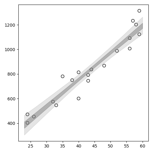
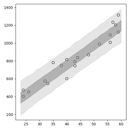
ベイズ予測区間
同様に作ればよいだろう.
まずはテスト(確認).
 1: import numpy as np
 2: import cmdstanpy
 3: import matplotlib.pyplot as plt
 4: import pandas as pd
 5: files=['model4-4-20220331192118_1.csv',
 6:        'model4-4-20220331192118_2.csv',
 7:        'model4-4-20220331192118_3.csv',
 8:        'model4-4-20220331192118_4.csv']
 9: fit = cmdstanpy.from_csv(path=files, method='sample')
10:
11: la = fit.stan_variables()  # { a:[...], b:[...], y_base:[[....],[....],....] }
12: X_new = range(23,61)
13:
14: y_new = la['y_new']
15: print(type(y_new))   # numpy.ndarray
16: print(len(y_new))    # 4000 列 (横に乱数が並んでいる感じ)
17: print(len(y_new[0])) # 38 行
18: df = pd.DataFrame()
19: for i in range(0,len(X_new)):
20:     df[i] = np.percentile(y_new[:,i], q=[2.5, 25, 50, 75, 97.5])
21: df2 = df.T
22: df3 = df2.set_axis(['p2.5','p25','p50','p75','p97.5'], axis='columns')
23: print(df3.head(5))
<class 'numpy.ndarray'>
4000
38
         p2.5        p25       p50        p75       p97.5
0  198.123700  326.81750  386.4070  447.93825  574.349600
1  212.061950  346.84150  408.3980  470.50200  598.318850
2  242.332525  367.20725  426.5785  487.02275  620.522400
3  268.728025  388.85600  452.0190  511.67625  638.447125
4  286.956400  411.82775  470.9350  533.02350  651.108675
 1: import numpy as np
 2: import cmdstanpy
 3: import matplotlib.pyplot as plt
 4: import pandas as pd
 5: d = pd.read_csv("data-salary.txt",header=0)
 6: X = d['X']
 7: Y = d['Y']
 8: files=['model4-4-20220331192118_1.csv',
 9:        'model4-4-20220331192118_2.csv',
10:        'model4-4-20220331192118_3.csv',
11:        'model4-4-20220331192118_4.csv']
12: fit = cmdstanpy.from_csv(path=files, method='sample')
13:
14: la = fit.stan_variables()  # { a:[...], b:[...], y_base:[[....],[....],....] }
15: X_new = range(23,61)
16:
17: y_new = la['y_new']
18: df = pd.DataFrame()
19: for i in range(0,len(X_new)):
20:     df[i] = np.percentile(y_new[:,i], q=[2.5, 25, 50, 75, 97.5])
21: df2 = df.T
22: df3 = df2.set_axis(['p2.5','p25','p50','p75','p97.5'], axis='columns')
23:
24: # X_new と df3 を使う
25:
26: fig = plt.figure(dpi=100, figsize=(5,5))
27: ax = fig.add_subplot(1,1,1)
28: ax.scatter(X,Y, marker='o', s=50, facecolor='None', edgecolors='black')
29: ax.fill_between(X_new, df3['p2.5'], df3['p97.5'], color='gray',alpha=0.2)
30: ax.fill_between(X_new, df3['p25'], df3['p75'],    color='gray',alpha=0.5)
31: plt.tight_layout()
32:
33: fname = 'fig4-8-right_py.png'
34: fig.show()
35: fig.savefig(fname)